Diffusion models I

Author

Simon Dirmeier <simd23 at pm dot me>

Published

June, 2022

Diffusion probabilistic models (DPMs), or generative diffusion processes, have attracted significant attention for generative modelling in the last couple of months. Similiarly to normalizing flows, DPMs model data iteratively via a set of transformations. The main idea of DPMs is to first add noise to a data set and then learn a reverse Markovian process that denoises the disrupted data and thus allows generating data from white noise. In this case study, we’ll reimplement the the vanilla model introduced in Sohl-Dickstein et al. (2015). To implement the models, we’ll use Jax, Haiku, Distrax and Optax.

import numpy as np
import pandas as pd

import jax
from jax import numpy as jnp, lax, nn, random
import optax
import haiku as hk
import distrax

import matplotlib.pyplot as plt
import seaborn as sns
import arviz as az
import palettes

sns.set(rc={"figure.figsize": (6, 3)}) 
sns.set_style("ticks", {'font.family': 'serif', 'font.serif': 'Merriweather'})
palettes.set_theme()

Diffusion models

We briefly discuss diffusion probabilistic models as introduced in Sohl-Dickstein et al. (2015). For details, please refer to the original paper or Ho et al. (2020). Diffusion models are latent variable models of the form

p_{θ} (y) = \int p_{θ} (y, z_{1 : T}) d z_{1 : T}

The above marginal is obtained by integrating over latent variables $z_{1 : T}$ which have the same dimensionality as the data $y$ . The joint distribution $p_{θ} (y, z_{1 : T})$ is defined via learned Markovian transitions

p_{θ} (y, z_{1 : T}) = p_{θ} (x ∣ z_{1}) t = 2 \prod T p_{θ} (z_{t - 1} ∣ z_{t}) p (z_{T})

where $p_{θ}$ is parameterized via a neural network. In comparison to other latent variable models, however, diffusion models start my assuming a forward process that iteratively corrupts a data set $x \sim q (y)$ via diffusions

q (z_{1 : T}, y) = q (y) q (z_{1} ∣ y) t = 2 \prod T q (z_{t} ∣ z_{t - 1})

that have a fixed schedule

q (z_{t} ∣ z_{t - 1}) = N (1 - β_{i} z_{t - 1}, β_{i} I)

Hence, diffusion probablistic models assume a fixed approximate posterior and learn the generative model $p_{θ}$ .

Implementation

Using the equations above, we can implement a DPM ourselves without much coding. With JAX and Haiku, a DPM could be implemented like that:

class DPM(hk.Module):
    def __init__(self, beta_schedule, reverse_process):
        super().__init__()
        self._reverse_process = reverse_process
        self.n_diffusions = len(beta_schedule)
        self.beta_schedule = beta_schedule

    def __call__(self, method="reverse_loc_and_log_scale", **kwargs):
        return getattr(self, method)(**kwargs)

    def _diffuse(self, z, beta):
        e = distrax.Normal(jnp.zeros_like(z), 1.0).sample(seed=hk.next_rng_key())
        z = jnp.sqrt(1.0 - beta) * z + jnp.sqrt(beta) * e
        return z

    def reverse_loc_and_log_scale(self, y):
        # forward diffusion
        zs = [y] + [None] * self.n_diffusions
        for i, beta in enumerate(self.beta_schedule):
            zs[i + 1] = self._diffuse(zs[i], beta)

        # reverse diffusion
        locs, log_scales = [None] * self.n_diffusions, [None] * self.n_diffusions
        for i in np.arange(self.n_diffusions - 1, -1, -1):
            loc, log_scale = jnp.split(self._reverse_process(zs[i + 1]), 2, axis=-1)
            locs[i] = loc
            log_scales[i] = log_scale

        return zs, locs, log_scales

    def reverse_diffusion(self, z):
        for _ in np.arange(self.n_diffusions):
            loc, log_scale = jnp.split(self._reverse_process(z), 2, axis=-1)
            e = distrax.Normal(jnp.zeros_like(z), 1.0).sample(seed=hk.next_rng_key())
            z = loc + jnp.exp(log_scale) * e
        return z

The function reverse_loc_and_log_scale first computes the forward process to sample all latent variables, and then, starting from the $z_{T}$ , computes the reverse process, or rather the locations and scales of each Gaussian transition, which are parameterized by a neural network.

Using Haiku, we construct and initialize a DPM like this:

n_diffusions = 5
beta_schedule = jnp.linspace(10e-4, 0.02, n_diffusions)

def _dm(method, **kwargs):
    reverse_process =  hk.Sequential([
        hk.Linear(256), jax.nn.leaky_relu,
        hk.Linear(256), jax.nn.leaky_relu,
        hk.Linear(256), jax.nn.leaky_relu,
        hk.Linear(2 * 2),
    ])
    return DPM(beta_schedule, reverse_process)(method, **kwargs)

diffusion = hk.transform(_dm)

In the model above, we are only using 5 diffusions. In practice, we should set this number higher to ensure that the distribution of last latent variable $z_{T}$ is approximately standard normal. However, as we will see later, optimizing an objective with $T = 1000$ is extremely inefficient and for demonstration we limit ourselves to only 5 diffusions.

Data

Let’s test the model on a synthetic data set. We sample data from the frequently found “nine Gaussians” distribution. The data set consists of nine fairly well separated Gaussian distributions which is a fairly difficult data set to learn the density of.

K = 9

means = jnp.array([-2.0, 0.0, 2.0])
means = jnp.array(jnp.meshgrid(means, means)).T.reshape(-1, 2)
covs = jnp.tile((1 / 16 * jnp.eye(2)), [K, 1, 1])

probs = distrax.Uniform().sample(seed=random.PRNGKey(23), sample_shape=(K,))
probs = probs / jnp.sum(probs)

d = distrax.MixtureSameFamily(
    distrax.Categorical(probs=probs),
    distrax.MultivariateNormalFullCovariance(means, covs)
)

n = 10000
y = d.sample(seed=random.PRNGKey(2), sample_shape=(n,))

The sampled data looks like this:

df = pd.DataFrame(np.asarray(y), columns=["x", "y"])
ax = sns.kdeplot(
    data=df, x="x", y="y", fill=True, cmap="mako_r"
)
ax.set_xlabel("$y_0$")
ax.set_ylabel("$y_1$")
plt.show()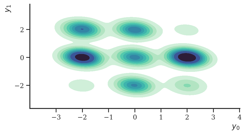

Before we train the model, we define some helper functions:

def timer(func):
    from timeit import default_timer
    def f(*args, **kwargs):
        start = default_timer()
        res = func(*args, **kwargs)
        stop = default_timer()
        print(f"Elapsed time: {stop - start}")
        return res
    return f

def _normal_from_beta(z, beta):
    return distrax.Independent(
        distrax.Normal(
            jnp.sqrt(1.0 - beta) * z,
            jnp.sqrt(beta)
        )
    )

def _normal(loc, log_scale):
    return distrax.Independent(
        distrax.Normal(
            loc,
            jnp.exp(log_scale)
        )
    )

def _std_normal(like):
    return distrax.Independent(
        distrax.Normal(
            jnp.zeros_like(like), jnp.ones_like(like)
        )
    )

ELBO

Training of diffusion models is performed by optimizing the usual evidence lower bound (ELBO):

lo g p_{θ} (y) \geq ELBO (q) = E_{q (z_{1 : T})} [lo g p_{θ} (y ∣ z_{1}) + i = 1 \sum T - 1 lo g p_{θ} (z_{i} ∣ z_{i + 1}) - i = 2 \sum T lo g q (z_{i} ∣ z_{i - 1}) + lo g p_{θ} (z_{T}) - lo g q (z_{1} ∣ y)]

We first initialize our diffusion model to get a pytree of parameters which we need for training.

params = diffusion.init(
    random.PRNGKey(2), 
    y=y, 
    method="reverse_loc_and_log_scale"
)

We optimize the ELBO using Optax. A single gradient step using Optax and the ELBO defined above looks, for instance, like this:

adam = optax.adamw(0.001)
opt_state = adam.init(params)

@jax.jit
def step(params, opt_state, y, rng):
    def loss_fn(params):
        zs, locs, log_scales = diffusion.apply(
            params, rng=rng, y=y, method="reverse_loc_and_log_scale"
        )

        # log likelihood p(y | z_1)
        log_pxz = _normal(locs[0], log_scales[0]).log_prob(y)

        kl = 0.0
        # note that: zs[0] == y
        for i in np.arange(1, len(zs)):
            # q(z_i | z_{i - 1}) where zs[0] = y
            lp_q = _normal_from_beta(zs[i - 1], beta_schedule[i - 1]).log_prob(zs[i])

            # p(z_i | z_{i + 1})
            if i != n_diffusions:
                lp_p = _normal(locs[i], log_scales[i]).log_prob(zs[i])
            # p(z_T)
            else:
                lp_p = _std_normal(zs[i]).log_prob(zs[i])

            kli = lp_q - lp_p
            kl += kli

        loss = -jnp.sum(log_pxz - kl)
        return loss

    loss, grads = jax.value_and_grad(loss_fn)(params)
    updates, new_opt_state = adam.update(grads, opt_state, params)
    new_params = optax.apply_updates(params, updates)
    return loss, new_params, new_opt_state

We use batch sizes of 128 and run the optimizer for 2000 epochs.

prng_seq = hk.PRNGSequence(42)
batch_size = 128
num_batches = y.shape[0] // batch_size
idxs = jnp.arange(y.shape[0])

@timer
def optim(params, opt_state, n_iter = 2000):    
    losses = [0] * n_iter
    for i in range(n_iter):
        loss = 0.0
        for j in range(batch_size):
            ret_idx = lax.dynamic_slice_in_dim(idxs, j * batch_size, batch_size)
            batch = lax.index_take(y, (ret_idx,), axes=(0,))
            batch_loss, params, opt_state = step(params, opt_state, batch, next(prng_seq))
            loss += batch_loss
        losses[i] = loss
    return params, losses

params, losses = optim(params, opt_state)
losses = jnp.asarray(losses)

This took quite some time even though we only used five diffusion steps. It also demonstrates why this objective is not very efficient to compute and prohibits a larger number of diffusions. Before we derive a more efficient objective, let’s have a look at some plots and if training actually worked.

Let’s have a look if the ELBO converged:

ax = sns.lineplot(
    data=pd.DataFrame({"y": np.asarray(losses), "x": range(len(losses))}),
    y="y", x="x",
    color='black'
)
ax.set(
    xlabel="", ylabel="-ELBO",
    xticks=[], xticklabels=[],
    yticks=[], yticklabels=[]
)
plt.show()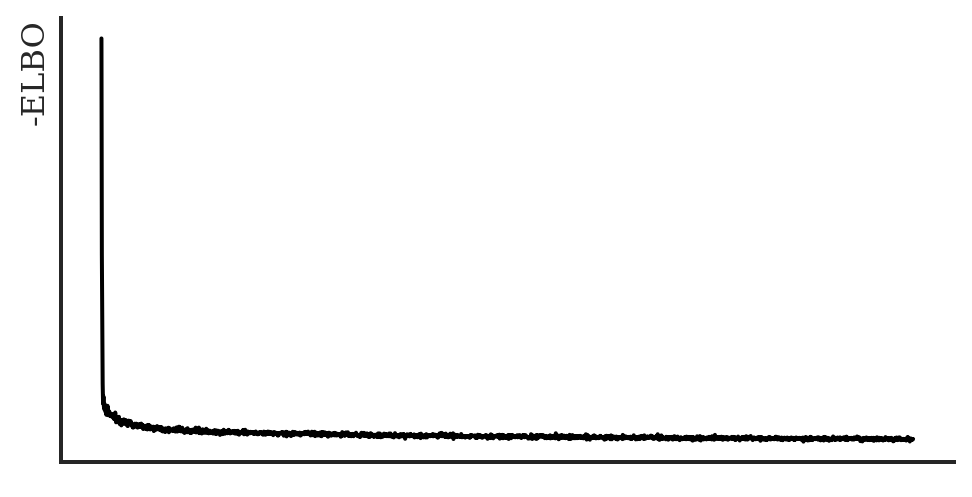

Having trained the model, we can sample from the diffusion model like this:

prior = distrax.Normal(jnp.zeros(2), jnp.ones(2))
z =  prior.sample(
    seed=random.PRNGKey(33),
    sample_shape=(5000,)
)
y_hat = diffusion.apply(
    params, rng=random.PRNGKey(1), 
    z=z, method="reverse_diffusion"
)

ax = sns.kdeplot(
    data=pd.DataFrame(np.asarray(y_hat), columns=["x", "y"]),
    x="x", y="y", fill=True, cmap="mako_r"
)
ax.set(xlabel="$y_0$", ylabel="$y_1$")
plt.show()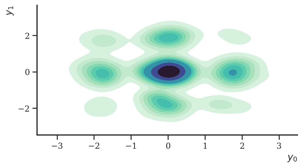

But for the sake of demonstration, this worked nicely! Visually, the estimated density is somewhat close to the original data set. To improve it, we could, for instance, increase the number of diffusions or use a more suitable network architecture.

A better objective

Given this simple neural network architecture and low sample size, training the objective took inacceptably much time. We can, however, use the following insight to define an objective that is easier to train. Since the forward transitions are all Gaussians, we can analytically integrate out intermediate steps, yielding:

q (z_{t} ∣ y) = N (α ˉ_{t} y, (1 - α ˉ_{t}) I)

Using Bayes rule, we can in addition derive the posterior of this process using:

q (z_{t - 1} ∣ z_{t}, y) = \frac{q ( z _{t} ∣ z _{t - 1} , y ) q ( z _{t - 1} ∣ y )}{q ( z _{t} ∣ y )} = N (μ ~_{t} (z_{t}, y), β ~_{t} I)

where

μ ~_{t} (z_{t}, y) = \frac{α ˉ _{t - 1} β _{t}}{1 - α ˉ _{t}} y + \frac{α ( 1 - α ˉ _{t - 1} )}{1 - α ˉ _{t}} z_{t}

and

β ~_{t} = \frac{1 - α ˉ _{t - 1}}{1 - α ˉ _{t}} β_{t}

Plugin these derivations into the ELBO gives us the following:

E_{q} [lo g p_{θ} (y ∣ z_{1}) - t = 2 \sum T KL [q (z_{t - 1} ∣ z_{t}, y), p_{θ} (z_{t - 1} ∣ z_{t})] - KL [q (z_{T} ∣ y), p_{θ} (z_{T})]]

Instead of sampling all T $z_{i}$ s, we can instead only optimize the first and the last part and one summand of the sum over the $t$ s

E_{q, t \sim U} [lo g p_{θ} (y, z_{1}) - KL [q (z_{t - 1} ∣ z_{t}, y), p_{θ} (z_{t - 1} ∣ z_{t})] - KL [q (z_{T} ∣ y), p_{θ} (z_{T})]]

In addition, if we reparameterize $z_{t}$ , we get

E_{q (y), t \sim U, p (ϵ_{t}), p (ϵ_{T})} [lo g p_{θ} (y, z_{1}) - KL [q (z_{t - 1} ∣ z_{t}, y), p_{θ} (z_{t - 1} ∣ z_{t})] - KL [q (z_{T} ∣ y), p_{θ} (z_{T})]]

In order to compute $q (z_{t} ∣ y)$ and $q (z_{t - 1} ∣ z_{t}, y)$ we update our DPM class:

class DPM(hk.Module):
    def __init__(self, beta_schedule, reverse_process):
        super().__init__()
        self._reverse_process = reverse_process
        self.n_diffusions = len(beta_schedule)
        self.beta_schedule = beta_schedule

    def __call__(self, method="reverse_process", **kwargs):
        return getattr(self, method)(**kwargs)

    def reverse_diffusion(self, z):
        for _ in np.arange(self.n_diffusions):
            loc, log_scale = jnp.split(self._reverse_process(z), 2, axis=-1)
            e = distrax.Normal(jnp.zeros_like(z), 1.0).sample(seed=hk.next_rng_key())
            z = loc + jnp.exp(log_scale) * e
        return z

    def _alpha_bar(self):
        alphas = 1.0 - self.beta_schedule
        alphas_bar = jnp.cumprod(alphas)
        return alphas_bar

    def _beta_tilde(self, t):
        alphas_bar = self._alpha_bar()
        return (1.0 - alphas_bar[t - 1]) / (1.0 - alphas_bar[t]) * self.beta_schedule[t]

    def reverse_process(self, z):
        loc, log_scale = jnp.split(self._reverse_process(z), 2, axis=-1)
        return distrax.Independent(
            distrax.Normal(loc, jnp.exp(log_scale)), 1
        )

    def forward_process(self, y, t):
        alphas_bar = self._alpha_bar()
        return distrax.Independent(
            distrax.Normal(
                jnp.sqrt(alphas_bar[t]) * y,
                jnp.repeat(jnp.sqrt(1.0 - alphas_bar[t]), y.shape[-1])
            ), 1
        )

    def sample_forward_process(self, y, t, epsilon=None):
        alphas_bar = self._alpha_bar()
        if epsilon is None:
            z = distrax.MultivariateNormalDiag(
                jnp.sqrt(alphas_bar[t]) * y,
                jnp.repeat(1.0 - alphas_bar[t], y.shape[-1])
            ).sample(seed=hk.next_rng_key())
        else:
            z = jnp.sqrt(alphas_bar[t]) * y + jnp.sqrt(1.0 - alphas_bar[t]) * epsilon
        return z

    def posterior_forward_process(self, y, zt, t):
        alphas = 1.0 - self.beta_schedule
        alphas_bar = self._alpha_bar()
        beta_tilde = self._beta_tilde(t)

        lhs = (jnp.sqrt(alphas_bar[t - 1]) * self.beta_schedule[t])
        lhs = lhs / (1.0 - alphas_bar[t]) * y

        rhs = jnp.sqrt(alphas[t]) * (1.0 - alphas_bar[t - 1])
        rhs = rhs / (1.0 - alphas_bar[t]) * zt

        return distrax.Independent(
            distrax.Normal(
                lhs + rhs,
                jnp.repeat(jnp.sqrt(beta_tilde), y.shape[-1])
            ), 1
        )

Since our new ELBO consists only of three terms, we can increase the number of diffusions. Here, we set it to 100:

n_diffusions = 100
beta_schedule = jnp.linspace(10e-4, 0.02, n_diffusions)

Training the ELBO is similar to the above. We first define the model again:

def _dm(method, **kwargs):
    reverse_process = hk.Sequential([
        hk.Linear(256), jax.nn.leaky_relu,
        hk.Linear(256), jax.nn.leaky_relu,        
        hk.Linear(256), jax.nn.leaky_relu,        
        hk.Linear(2 * 2),
    ])
    return DPM(beta_schedule, reverse_process)(method, **kwargs)

diffusion = hk.transform(_dm)
params = diffusion.init(
    random.PRNGKey(23),
    z=y,
    method="reverse_process"
)

Then, we define our updated objective:

adam = optax.adamw(0.001)
opt_state = adam.init(params)
np.random.seed(2)

@jax.jit
def step(params, opt_state, y, rng):
    def loss_fn(params):
        t = np.random.choice(np.arange(1, n_diffusions))

        ## compute the last term: KL between priors
        q_z_T = diffusion.apply(
            params, rng=rng, y=y, t=n_diffusions - 1, method="forward_process"
        )
        p_z_T = distrax.Independent(
            distrax.Normal(jnp.zeros_like(y), 1), 1
        )
        # KL q(z_T | y) || p(z_T)
        kl_T = q_z_T.kl_divergence(p_z_T)

        ## compute the middle term: KL between two adjacent t's
        sample_rng, new_rng = random.split(rng)
        e_t = distrax.Normal(jnp.zeros_like(y), 1.0).sample(seed=sample_rng)        
        z_t = diffusion.apply(
            params, rng=rng, y=y, t=t, epsilon=e_t,
            method="sample_forward_process"
        )
        q_z_tm1 = diffusion.apply(
            params, rng=rng, y=y, zt=z_t, t=t,
            method="posterior_forward_process"
        )
        p_z_tm1 = diffusion.apply(
            params, rng=rng, z=z_t, method="reverse_process"
        )
        # KL q(z{t - 1} | Z_t, Y) || p(z_{t - 1} | z_t)
        kl = q_z_tm1.kl_divergence(p_z_tm1)

        ## compute the first term: log likeihood
        sample_rng, new_rng = random.split(new_rng)
        e_1 = distrax.Normal(jnp.zeros_like(y), 1.0).sample(seed=sample_rng)
        z_1 = diffusion.apply(
            params, rng=rng, y=y, t=0, epsilon=e_1, method="sample_forward_process"
        )
        p_z_1 = diffusion.apply(
            params, rng=rng, z=z_1, method="reverse_process"
        )        
        # log likelihood P(Y | Z_1)
        log_pxz = p_z_1.log_prob(y)
        
        loss = -jnp.sum(log_pxz - kl - kl_T)
        return loss

    loss, grads = jax.value_and_grad(loss_fn)(params)
    updates, new_opt_state = adam.update(grads, opt_state, params)
    new_params = optax.apply_updates(params, updates)
    return loss, new_params, new_opt_state

Finally, we train the model. The training procedure is exactly the same as above.

prng_seq = hk.PRNGSequence(1)
batch_size = 128
num_batches = y.shape[0] // batch_size
idxs = jnp.arange(y.shape[0])

@timer
def optim(params, opt_state, n_iter = 2000):    
    losses = [0] * n_iter
    for i in range(n_iter):
        loss = 0.0
        for j in range(batch_size):
            ret_idx = lax.dynamic_slice_in_dim(idxs, j * batch_size, batch_size)
            batch = lax.index_take(y, (ret_idx,), axes=(0,))
            batch_loss, params, opt_state = step(params, opt_state, batch, next(prng_seq))
            loss += batch_loss
        losses[i] = loss
    return params, losses

params, losses = optim(params, opt_state)
losses = jnp.asarray(losses)

Training this objective is significantly faster than the original one, despite increasing the number of diffusions. Let’s have a look at the ELBO again:

ax = sns.lineplot(
    data=pd.DataFrame({"y": np.asarray(losses), "x": range(len(losses))}),
    y="y", x="x",
    color='black'
)
ax.set(
    xlabel="", ylabel="-ELBO",
    xticks=[], xticklabels=[],
    yticks=[], yticklabels=[]
)
plt.show()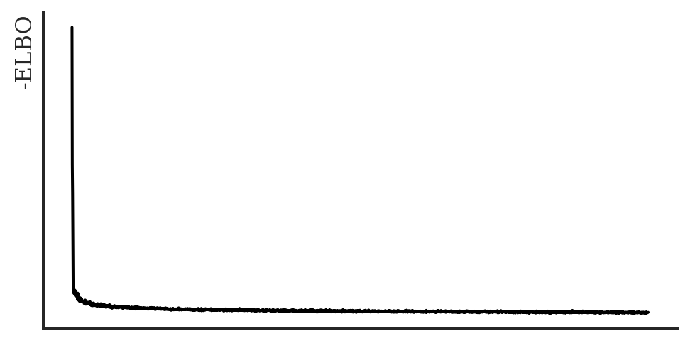

In the end, let’s also sample some data.

prior = distrax.Normal(jnp.zeros(2), jnp.ones(2))
z = prior.sample(
    seed=random.PRNGKey(33),
    sample_shape=(5000,)
)
y_hat = diffusion.apply(
    params, rng=random.PRNGKey(1), 
    z=z, method="reverse_diffusion"
)

ax = sns.kdeplot(
  data=pd.DataFrame(np.asarray(y_hat), columns=["x", "y"]),
  x="x", y="y", fill=True, cmap="mako_r"
)
ax.set(xlabel="$y_0$", ylabel="$y_1$")
plt.show()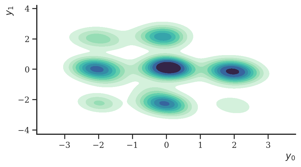

As before, the density of the data was estimated fairly well given the simple model architecture.

Conclusion

DPMs are an exciting new class of models for generative modelling and density estimation. Even though the model was originally published in 2015 already, recent interest was (afaict) mainly sparked by the follow-up papers by Ho et al. (2020) and Dhariwal and Nichol (2021) which demonstrated that DPMs are SOTA generative models, e.g., in image generation. The next case-study will demonstrate the improvements made by Ho et al. (2020).

References

Dhariwal, P. and Nichol, A. (2021). Diffusion Models Beat GANs on Image Synthesis. Advances in Neural Information Processing Systems, 34, 8780–8794.

Ho, J., Jain, A., and Abbeel, P. (2020). Denoising Diffusion Probabilistic Models. Advances in Neural Information Processing Systems, 33, 6840–6851.

Sohl-Dickstein, J., Weiss, E., Maheswaranathan, N., and Ganguli, S. (2015). Deep Unsupervised Learning using Nonequilibrium Thermodynamics. International Conference on Machine Learning, 2256–2265. PMLR.