Probabilistic forecast reconciliation

In this case study we implement and test methods for probabilistic forecast reconciliation based on the recent papers by Panagiotelis et al. (2022) and Zambon et al. (2022).

Forecast reconciliation is often found in hierarchical time series analysis scenarios, i.e., where time series can be (dis-)aggregated linearly by various attributes in a hierarchical way. For instance, consider a scenario in retail forecasting where we are interested in predicting the number of sold books per day. Forecasts are often required for all levels of a hierarchy, i.e., for the time series on the very bottom (e.g., cities), the inner nodes of a hierarchy (e.g., regions, counties) and the root node of the hierarchy (e.g., country) and it is natural to want the forecasts to add up in the same way as the data. For example, forecasts of sales per city should add up to forecasts of sales per canton, etc. In this case the hierarchy is induced by the granularity of the location as exemplified by the tree below:

import networkx as nx
import matplotlib.pyplot as plt
from networkx.drawing.nx_pydot import graphviz_layout

G = nx.DiGraph()
G.add_edge("Switzerland", "Greater-Zurich")
G.add_edge("Switzerland", "Ticino")
G.add_edge("Greater-Zurich", "Zurich")
G.add_edge("Greater-Zurich", "Winterthur")
G.add_edge("Ticino", "Lugano")
G.add_edge("Ticino", "Bellinzona")

pos = {
    "Switzerland": (4, 1), 
    "Greater-Zurich": (6, 0.5),
    "Zurich": (5, 0),
    "Winterthur": (7, 0),
    "Ticino": (2, 0.5), 
    "Lugano": (1, 0),
    "Bellinzona": (3, 0),
}
options = {
    "node_color": "white",
    "edgecolors": "black",
    "linewidths": 0,
    "width": 2,
}

_ = plt.figure(figsize=(6, 3))
nx.draw_networkx(G, pos=pos, **options)
plt.axis("off")
plt.show()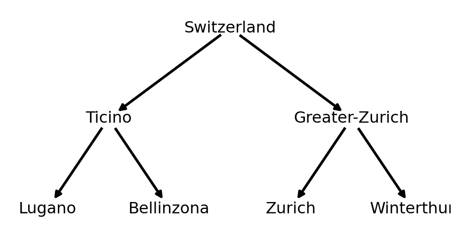

Propabilistic forecast reconciliation aims at generating coherent probabilistic forecasts over all levels of the hierarchy.

Before we implement the two methods introduced in Panagiotelis et al. (2022) and Zambon et al. (2022), we briefly introduce probabilistic reconciliation. We then implement and test the two methods where we use GPJax to produce forecasts with Gaussian processes. I bundled the code for this case study as a Python package called reconcile which can be found here.

import distrax
import gpjax as gpx
import jax
from jax import numpy as jnp
from jax import random
import numpy as np
import optax
import pandas as pd
import pathlib

from reconcile.forecast import Forecaster
from reconcile.grouping import Grouping
from reconcile.probabilistic_reconciliation import ProbabilisticReconciliation

import matplotlib.pyplot as plt
import seaborn as sns
import palettes

from jax.config import config
config.update("jax_enable_x64", True)

Probabilistic reconciliation

Denote with ${\mathbf{b}}^t\in {\mathbb{R}}^P$ a vector of observations of “bottom-level” time series at time $t$ and with $y_n^t$ an observation of node $n$ at time $t$. For instance, in the example above ${\mathbf{b}}^t=\{y_{\text{Lugano}}^t,y_{\text{Bellinzona}}^t,y_{\text{Zurich}}^t,y_{\text{Winterthur}}^t\}$. We can aggregate the bottom level observations such that the parents of nodes are sums of their children, via an summing matrix $\mathbf{S}\in \{0,1{\}}^{Q\times P}$

where $\mathbf{S}$ defines the hierarchical structure of the time series. Again, as an example, for the hierarchy above

where $\mathbf{A}$ is called aggregation matrix, $\mathbf{I}$ is a diagonal matrix, and the vector ${\mathbf{y}}^t=\{y_{\text{Switzerland}}^t,y_{\text{Ticino}}^t,y_{\text{Greater-Zurich}}^t,y_{\text{Lugano}}^t,y_{\text{Bellinzona}}^t,y_{\text{Zurich}}^t,y_{\text{Winterthur}}^t\}$ contains all the time series over the hierarchy. When we generate forecasts $\hat{\mathbf{y}}$ for all of these timeseries, they might not cohere to the linear constraints induced by the hierarchy.

In a probabilistic (e.g., Bayesian) framework forecasts are available in the form of probability distributions. Following Zambon et al. (2022), we denote $\hat{\nu }\in \mathbb{P}({\mathbb{R}}^Q)$ the forecast distribution of $\hat{\mathbf{y}}$ and call it coherent ($\tilde{\nu }$) if $\text{supp}(\hat{\nu })$ is in a linear subspace $\mathcal{S}$ of dimension $P$ of ${\mathbb{R}}^Q$.

To find a coherent forecast distribution $\tilde{\nu }$, Panagiotelis et al. (2022) propose to fit a map $\psi :{\mathbb{R}}^Q\to \mathcal{S}$, such that $\tilde{\nu }={\psi }_{♯}\hat{\nu }$. Panagiotelis et al. (2022) use a simple linear transformation $\psi (\mathbf{y})=\mathbf{S}(\mathbf{d}+\mathbf{Wy})$ and fit it using an approximate energy score as objective.

Zambon et al. (2022) propose sampling from the reconciled base forecast density $\tilde{\pi }(\mathbf{b})$ of $\mathbf{b}$ via $\tilde{\pi }(\mathbf{b})\propto {\pi }_U(\mathbf{Ab}){\pi }_B(\mathbf{b})$ where $\mathbf{A}$ is the aggregation matrix, and ${\pi }_U$ and ${\pi }_B$ are the predictive densities of the upper level time series, i.e., the ones corresponding to the inner nodes and root, and bottom level time series.

For further details, please refer to the original publications.

Data

We will test the two methods on a finance data set, specifically stock index data of some constituents of the SP500 which we take from datahub and Kaggle.

Of the SP500, we somewhat arbitrarily picked some consituents from the health care and information technology industries and selected all entries from 2022 on. In that case the hierarchy consists of two levels, where “Health Care” and “Information Technology” are the parents of the different companies (which are leaves).

def preprocess():
    constituents_sp500 = pd.read_csv("./constituents.csv")
    constituents_sp500 = constituents_sp500[
        (constituents_sp500.Sector == "Health Care") |
        (constituents_sp500.Sector == "Information Technology")
    ]
    
    dfs = []
    for constituent in constituents_sp500.iterrows():
        path = f"./stocks/{constituent[1].Symbol}.csv"
        if pathlib.Path(path).exists():
            df = pd.read_csv(path)
            df["Sector"] = constituent[1].Sector
            df["Name"] = constituent[1].Name
            dfs.append(df)
    df = pd.concat(dfs)
    
    df_constituents = [
        "Illumina Inc", "Johnson & Johnson", "Pfizer Inc.", "Thermo Fisher Scientific", "Merck & Co.",
        "Activision Blizzard", "Boston Scientific", "Netflix Inc.", "Microsoft Corp.", "Seagate Technology"
    ]
    df = df[df.Name.isin(df_constituents)]

    df.Date = pd.to_datetime(df.Date, infer_datetime_format=True)
    df = df[df.Date > np.datetime64("2021-12-31")]
    
    return df

df = preprocess()

Let’s have a look at the different stock time series.

df["Standardized"] = df.groupby(
    ["Sector", "Name"]
)["Close"].transform(lambda x: (x - x.mean()) / x.std())
g = sns.FacetGrid(
    df,
    row="Sector",
    hue="Name",
    palette=sns.color_palette("crest"),
    sharex=False, 
    sharey=False,
    height=2.5, 
    aspect=3,
)
_ = g.map_dataframe(
    sns.lineplot, x="Date", y="Standardized", style="Name",
)
_ = g.set_axis_labels("", "Standardized index")
plt.show()
df = df.drop(columns="Standardized")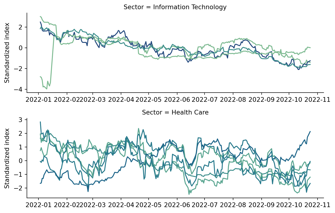

Before we try start forecasting these, we postprocess the data, e.g., by transforming the dates into numeric values and then extract them from the data frame as arrays.

def postprocess(df):
    df["Series"] = df["Sector"] + ":" + df["Name"]
    df = df[["Date", "Series", "Close"]]
    df = df.rename(columns={"Close": "Value"})
    df = df.pivot(index="Date", columns='Series', values='Value').reset_index()
    df = df.dropna()
    df.insert(0, "x", (df.Date - np.min(df.Date)) / (np.max(df.Date) - np.min(df.Date)))
    return df

def get_bottom_level_timeseries(df):
    x = df.x.values.reshape(1,  1, -1)
    b = df.drop(columns=["Date", "x"]).values.T
    b = b.reshape(1, *b.shape)
    return b, x

D = postprocess(df)
b, x = get_bottom_level_timeseries(D)

Using reconcile we can define a hierarchy (or more generally a grouping) using the Grouping class. To do so, we first create a ”:“-separated string for every bottom level time series that specifies the path of the time series to the root of the hierarchy.

hierarchy = list(D.drop(columns=["Date", "x"]).columns)
hierarchy

Since in our example, the hierarchy is very flat (only one inner level), the strings are only separated by one colon. For instance “Boston Scientific” is in the health care sector, hence we create an entry “Health Care:Boston Scientific”. We then create a grouping using the list of strings.

groups = pd.DataFrame({"hierarchy": hierarchy})
grouping = Grouping(groups)

Forecasts

Before we can probabilistically reconcile forecasts, we first need to generate probabilistic forecasts (yupp), or rather predictive distributions. We use GPJax’s Gaussian process implementations for this. Specifically, we fit a Gaussian process to every time series separately and then, in a post-processing step, reconcile those forecasts.

GPs are arguably not the best model here, but for the sake of demonstrating the two reconciliation methods it is fine, since we don’t aim to make perfectly accurate predictions here.

We first get all the time series, i.e, bottom and upper level time series, from the Grouping object.

all_timeseries = grouping.all_timeseries(b)
all_features = jnp.tile(x, [1, all_timeseries.shape[1], 1])

We then define a forecasting class. The class needs to inherit from Forecaster which is implemented in the Python package we developed for this case study. The class needs to provide a fit method that fits all of the time series, a posterior_predictive method which returns a posterior predictive distribution of all time series as distrax object, and a method predictive_posterior_probability that computes the probabilty of observing some event under the posterior predictive.

class GPForecaster(Forecaster):
    """Example implementation of a forecaster"""

    def __init__(self):
        self._models = []
        self._xs = None
        self._ys = None

    @property
    def data(self):
        """Returns the data"""
        return self._ys, self._xs

    def fit(self, rng_key, ys, xs):
        """Fit a model to each of the time series"""
        self._xs = xs
        self._ys = ys

        p = xs.shape[1]
        self._models = [None] * p
        for i in np.arange(p):
            x, y = xs[:, [i], :], ys[:, [i], :]
            # fit a model for each time series
            learned_params, D = self._fit_one(rng_key, x, y)
            # save the learned parameters and the original data
            self._models[i] = learned_params, D

    def _fit_one(self, rng_key, x, y):
        # here we use GPs to model the time series
        D = gpx.Dataset(X=x.reshape(-1, 1), y=y.reshape(-1, 1))
        posterior, likelihood = self._model(rng_key, D.n)

        parameter_state = gpx.initialise(posterior, key=rng_key)
        mll = jax.jit(posterior.marginal_log_likelihood(D, negative=True))

        optimiser = optax.adam(learning_rate=5e-2)
        inference_state = gpx.fit(mll, parameter_state, optimiser, n_iters=2000, verbose=False)
        learned_params, _ = inference_state.unpack()
        
        return learned_params, D

    @staticmethod
    def _model(rng_key, n):
        D = gpx.Dataset(X=x[0, 0].reshape(-1, 1), y=b[0, 0].reshape(-1, 1))
        kernel = gpx.RBF() + gpx.Matern32()
        prior = gpx.Prior(mean_function=gpx.Constant(), kernel=kernel)
        likelihood = gpx.Gaussian(num_datapoints=D.n)
        posterior = prior * likelihood
       
        return posterior, likelihood

    def posterior_predictive(self, rng_key, xs_test):
        """Compute the joint
        posterior predictive distribution of all timeseries at xs_test"""

        q = xs_test.shape[1]
        means = [None] * q
        covs = [None] * q
        for i in np.arange(q):
            x_test = xs_test[:, [i], :].reshape(-1, 1)
            learned_params, D = self._models[i]
            posterior, likelihood = self._model(rng_key, D.n)
            latent_distribution = posterior(learned_params, D)(x_test)
            predictive_dist = likelihood(learned_params, latent_distribution)
            means[i] = predictive_dist.mean()
            cov = jnp.linalg.cholesky(predictive_dist.covariance_matrix)
            covs[i] = cov.reshape((1, *cov.shape))

        # here we stack the means and covariance functions of all
        # GP models we used
        means = jnp.vstack(means)
        covs = jnp.vstack(covs)

        # here we use a single distrax distribution to model the predictive
        # posterior of _all_ models
        posterior_predictive = distrax.MultivariateNormalTri(means, covs)
        return posterior_predictive

    def predictive_posterior_probability(
        self, rng_key, ys_test, xs_test
    ):
        """Compute the log predictive posterior probability of an observation"""
        preds = self.posterior_predictive(rng_key, xs_test)
        lp = preds.log_prob(ys_test)
        return lp

The time series have a total length of 204 of which we take the first 200 for training.

all_timeseries.shape

idx_train = 200

We then fit the GPForecaster to the time series.

forecaster = GPForecaster()
forecaster.fit(
    random.PRNGKey(1), all_timeseries[:, :, :idx_train], all_features[:, :, :idx_train]
)

As baseline to the two reconciliation methods, we also sample from the posterior predictive of the base forecasts.

y_predictive = forecaster.posterior_predictive(
    random.PRNGKey(1), all_features
)
y_predictive_samples = y_predictive.sample(
    seed=random.PRNGKey(2), sample_shape=(1000,)
)
b_predictive_mean = jnp.mean(y_predictive_samples, axis=0, keepdims=True)[:, 3:, :]

D_pred = pd.DataFrame(b_predictive_mean[0].T, columns=hierarchy)
D_pred.insert(0, "Data type", "Predicted")
D_pred.insert(1, "Date", D.Date)

Next we use a method similar to Panagiotelis et al. (2022) to reconcile the base forecasts.

recon = ProbabilisticReconciliation(grouping, forecaster)
b_pred_fit_recon = recon.fit_reconciled_posterior_predictive(
   random.PRNGKey(1), all_features, n_samples=1000, n_iter=1000,
)
b_pred_fit_recon_mean = jnp.mean(b_pred_fit_recon, axis=0, keepdims=True)

D_fit_recon = pd.DataFrame(b_pred_fit_recon_mean[0].T, columns=hierarchy)
D_fit_recon.insert(0, "Data type", "Reconciled via optimization")
D_fit_recon.insert(1, "Date", D.Date)

We use the MCMC-based method in Zambon et al. (2022) for sampling-based reconciliation.

b_pred_sample_recon = recon.sample_reconciled_posterior_predictive(
   random.PRNGKey(1), all_features
)
b_pred_sample_recon_mean = jnp.mean(
    jnp.mean(b_pred_sample_recon, axis=1, keepdims=False), axis=0, keepdims=True
)

D_sample_recon = pd.DataFrame(b_pred_sample_recon_mean[0].T, columns=hierarchy)
D_sample_recon.insert(0, "Data type", "Reconciled via sampling")
D_sample_recon.insert(1, "Date", D.Date)

Let’s visualize the results. We first aggregate all forecasts in a data frame and then plot the original data, the base forecasts and the two recconciled forecasts.

D_all = D.drop(columns="x")
D_all.insert(0, "Data type", "Real")
D_all = pd.concat([D_all, D_pred, D_sample_recon, D_fit_recon], axis=0)
D_all = D_all.melt(id_vars=["Date", "Data type"])
D_all[['Sector','Name']] = D_all.variable.str.split(":",expand=True)

g = sns.FacetGrid(
    D_all,
    col="Name",
    col_wrap=2,
    sharex=False, 
    sharey=False,
    height=1.75,
    aspect=2
)
_ = g.map_dataframe(
    sns.lineplot, x="Date", y="value", style="Data type", color="black"
)
_ = g.tight_layout()
_ = g.set_axis_labels("", "Index")
_ = g.set(xticklabels=[])
_ = g.add_legend()
plt.show()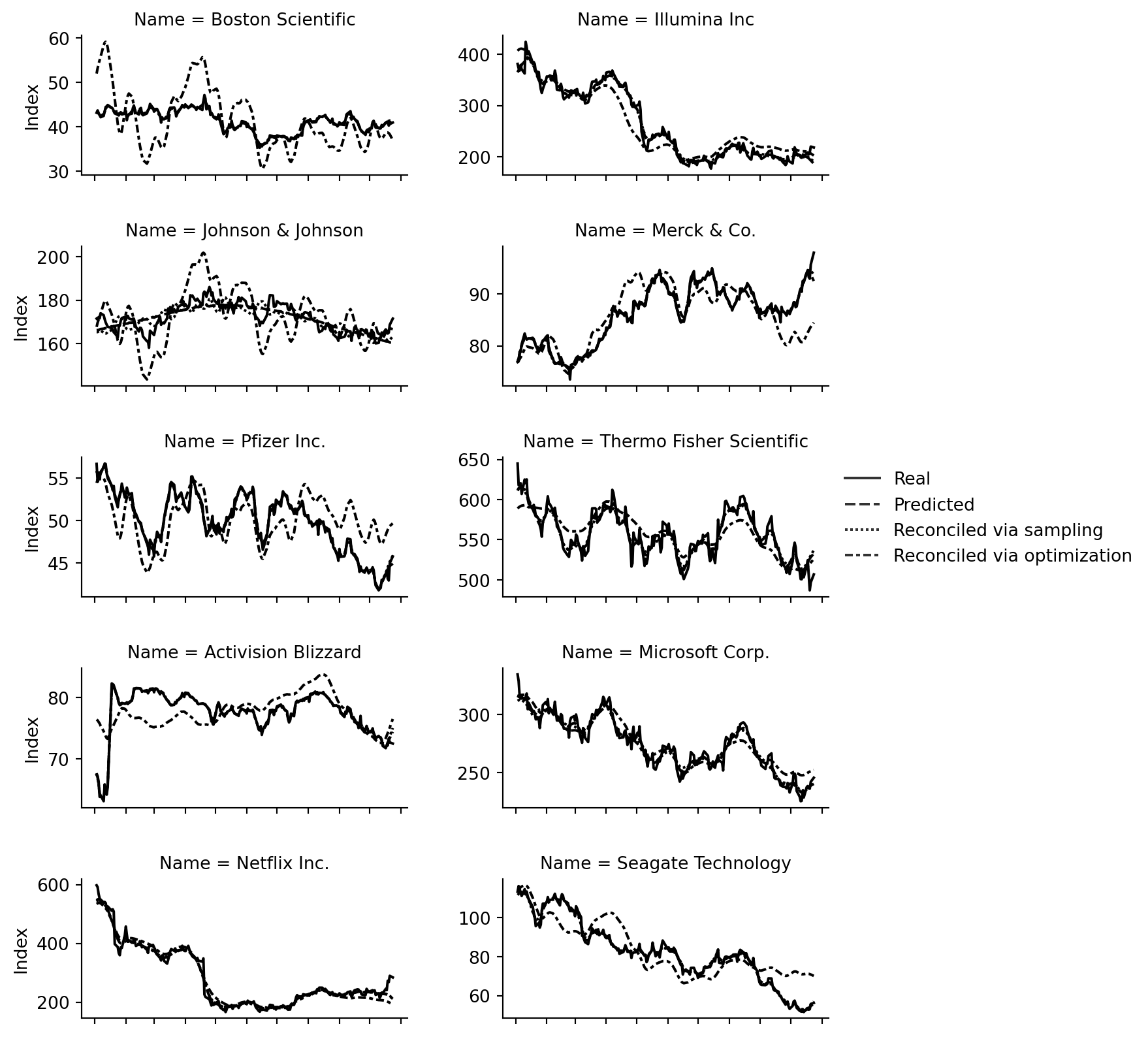

The results look decent for some of the time series and even worse than the base forecasts for others. Given that the time series don’t present clear trends or saisonalities, the task was arguably a very difficult one though.

Conclusion

This case study implemented and tested two methods based on recent papers on probabilstic forecast reconciliation. We evaluated the methods (superficially) on stock-index time series data of the SP500 with mixed results. Stock-index data is notoriously hard to forecast due to their (apparent) stationarity, and the evaluation was consequently not very meaningful, but rather intended to understand probabilistic reconciliation methods better.

The methods demonstrated above are implemented in a Python package called reconcile which can be found on PyPI and GitHub.

References

Panagiotelis, A., Gamakumara, P., Athanasopoulos, G., and Hyndman, R. J. (2022). Probabilistic forecast reconciliation: Properties, evaluation and score optimisation. European Journal of Operational Research.

Zambon, L., Azzimonti, D., and Corani, G. (2022). Probabilistic reconciliation of forecasts via importance sampling. arXiv preprint arXiv:2210.02286.